D R Markdown

An R Markdown (.Rmd) file will allow you to integrate your R commands, output and written work in one document. You write your R code and explanations in the .Rmd file, the knit the document to a Word, HTML, or pdf file. A basic R Markdown file has the following elements:

Header: this is the stuff in between the three dashes --- located at the top of your .Rmd file. A basic header should specify your document title, author and output type (e.g. word_document).
Written work: Write up your work like you would in any word/google doc. Formatting is done with special symbols. E.g. to bold a word or phrase, place two asterisks ** at the start and end of the word or phrase (with no spaces). To get section headers use one or more hash tags # prior to the section name.
R code: Your R commands are contained in one or more chunks that contains one or more R commands. A chunk starts with three backticks (to the left of your 1 key) combined with {r} and a chunk ends with three more backticks. See the image below for an example of a chunk that reads in the data files HollywoodMovies2011.csv.

A R chunk that reads in a data file

Important!! A common error that students run into when first using R Markdown is forgetting to put the read.csv command in their document. An R Markdown document must contain all commands needed to complete an analysis. This includes reading in the data! Basically, what happens during the knitting process is that a fresh version of an Rstudio environment is created that is completely separate from the Rstudio you see running in front of you. The R chunks are run in this new environment, and if you will encounter a Markdown error if you, say, try to use the movies data frame without first including the read.csv chunk shown in Figure 1.

D.1 How to write an R Markdown document

Write your commands in R chunks, not in the console. Run chunk commands using the suggestions in the Hints section below.
Knit your document often. This allows you to catch errors/typos as you make them.
You can knit a .Rmd by pressing the Knit button at the top of the doc. You can change output types (e.g. switch from HTML to Word) by typing in the preferred doc type in the header, or by using the drop down menu option found by clicking the down triangle to the right of the Knit button.
You can run a line of code in the R console by putting your cursor in the line and selecting Run > Run Selected Line(s).
You can run all commands in a chunk by clicking the green triangle on the right side of the chunk.
URLs can be embeded between < and > symbols.
The image below shows a quick scrolling menu that is available by clicking the double triangle button at the bottom of the .Rmd. This menu shows section headers and available chunks. It is useful for navagating a long .Rmd file.

Quick scroll through Markdown document

D.2 Changing R Markdown chunk evaluation behavior

The default setting in Rstudio when you are running chunks is that the “output” (numbers, graphs) are shown “inline” within the Markdown Rmd. For a variety of reasons, my preference is to have commands run in the console. To see the difference between these two types of chunk evaluation option, you can change this setting as follows:

Select Tools > Global Options.
Click the R Markdown section and uncheck (if needed) the option Show output inline for all R Markdown documents.
Click OK.

Now try running R chunks in the .Rmd file to see the difference. You can recheck this box if you prefer the default setting.

D.3 Creating a new R Markdown document

I suggest using old .Rmd HW file as a template for a new HW assignment. But if you want to create a completely new docment:

Click File > New File > R Markdown….
A window like the one shown below should appear. The default settings will give you a basic Markdown (.Rmd) file that will generate an HTML document. Click OK on this window.

Opening a Markdown document

You should now have an “Untitled1” Markdown file opened in your document pane of Rstudio. Save this file, renamed as “FirstMarkdown.Rmd,” somewhere on your computer. (Ideally in a Stat230 folder!) On Mirage, save the file in the default location (which is your account folder on the mirage server).
Now click the Knit HTML button on the tool bar at the top of your Markdown document. This will generate a “knitted” (compiled) version of this document. Check that there is now an HTML file named “FirstMarkdown.html” in the same location as your “FirstMarkdown.Rmd” file.

D.4 Extra: Graph formatting

The markdown .Rmd for this graph formatting section is linked here: https://kstclair.github.io/Rmaterial/Markdown/Markdown_GraphFormatting.Rmd

The data set Cereals contains information on cereals sold at a local grocery store.

# load the data set 
Cereals <- read.csv("http://math.carleton.edu/Stats215/RLabManual/Cereals.csv")

D.4.1 Adding figure numbers and captions

To add captions to the figures you make you need to add the argument fig.cap="my caption" to your R chunk that creates the figure. If you have two or more figures created in the R chunk then give the fig.cap argument a vector of captions.

If you are knitting to a pdf, you don’t need to add “Figure 1,” etc. numbering to the figure captions (they will be numbered automatically). For HTML and Word output types, you need to manually number figures.

D.4.2 Resizing graphs in Markdown

Suppose we want to create a boxplot of calories per gram grouped by cereal type and a scatterplot of calories vs. carbs per gram. Here are the basic commands without any extra formatting that create Figures 1 and 2:

```{r, fig.cap="Figure 1: Distributions of calories per gram by cereal type"}
boxplot(calgram ~ type, data=Cereals, main="Calories by type", ylab="Calories per gram")
```

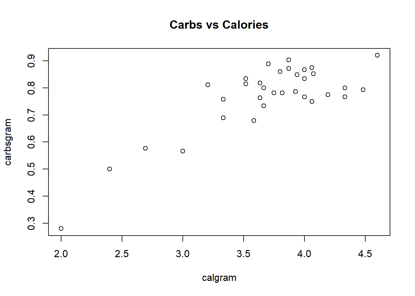
Figure D.1: Distributions of calories per gram by cereal type

```{r, fig.cap="Figure 2: Calories vs. Carbs per gram"}
plot(carbsgram ~ calgram, data=Cereals, main="Carbs vs Calories")
```

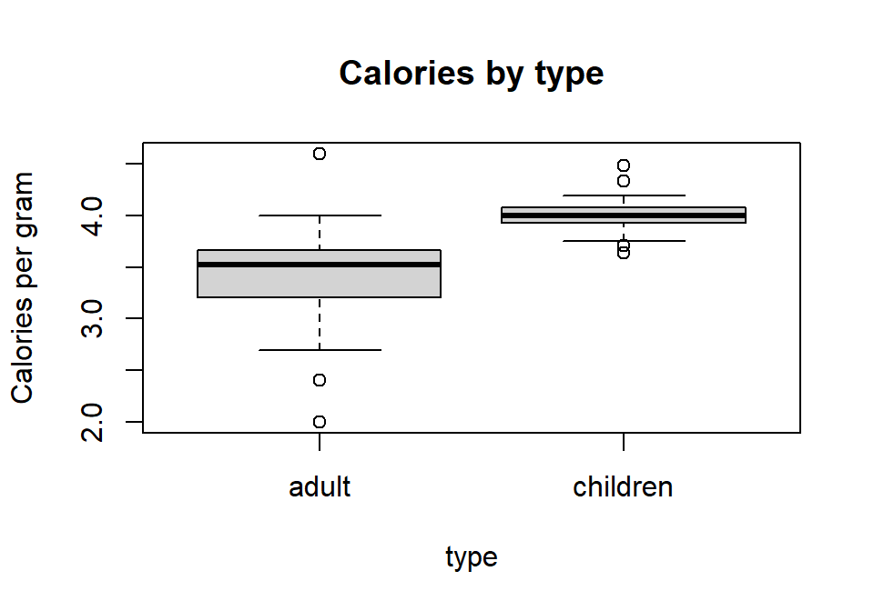
Figure D.2: Calories vs. Carbs per gram

We can add fig.height and fig.width parameters to the Markdown R chunk to resize the output size of the graph. The size inputs used here are a height of 3.5 inches and a width of 6 inches. The command below creates Figures 3 and 4.

```{r, fig.height=3.5, fig.width=5, fig.cap=c("Figure 3: Distributions of calories per gram by cereal type","Figure 4: Calories vs. Carbs per gram")}
boxplot(calgram ~ type, data=Cereals, main="Calories by type", ylab="Calories per gram")
plot(carbsgram ~ calgram, data=Cereals, main="Carbs vs Calories")
```

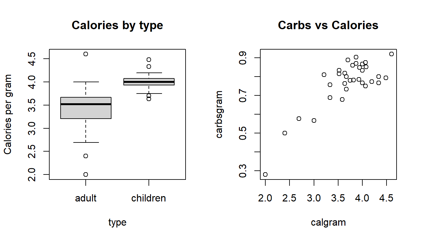
boxplot(calgram ~ type, data=Cereals, main="Calories by type", ylab="Calories per gram")

Figure D.3: Distributions of calories per gram by cereal type

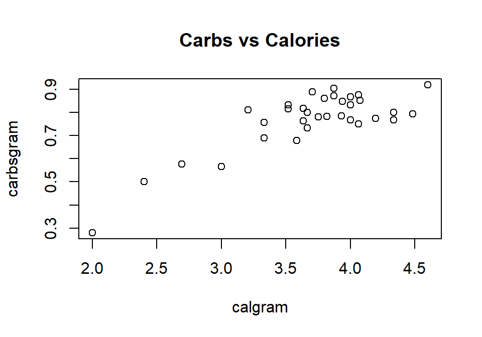
plot(carbsgram ~ calgram, data=Cereals, main="Carbs vs Calories")

Figure D.4: Calories vs. Carbs per gram

D.4.3 Changing graph formatting in R

You can use the par command to change R’s graphical parameter settings for plots that are not made from ggplot2. There are many options that can be changed, but one of the most useful is to change the layout of the graphical output display. The argument mfrow (multi-frame row) is given a vector c(nr, nc) that draws figures in an nr (number of rows) by nc (number of columns) array. We can arrange our two graphs in a 1 by 2 display (1 row, 2 columns) with the command:

par(mfrow=c(1,2))
boxplot(calgram ~ type, data=Cereals, main="Calories by type", ylab="Calories per gram")
plot(carbsgram ~ calgram, data=Cereals, main="Carbs vs Calories")

Figure D.5: Distribution of calories per gram by cereal type and calories vs. carbs per gram.

D.4.4 Hiding R commands

You can omit R commands from your final document by adding echo=FALSE to your R chunk argument. Any output produced by your command (graphical or numerical) will still be displayed. For example, the following command creates Figure 6, a boxplot of carbs per gram by cereal type.

```{r, echo=FALSE, fig.cap="Figure 6: Distributions of calories per gram and shelf placement by cereal type", fig.height=3, fig.width=4}
boxplot(carbsgram ~ type, data=Cereals, main="Carbs by type", ylab="Carbs per gram")
```

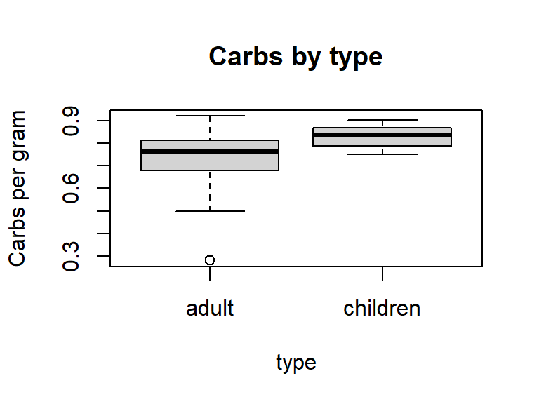
Figure D.6: Distributions of calories per gram and shelf placement by cereal type

D.4.5 Global changes in graph format

The R chunk options that control graph sizes and output features (like echo) can be set globally for all R chunks either in the header (like with fig.caption) or in an opts_chunk$set() command at the start of the .Rmd file. I usually opt for setting global features with the opts_chunk command which you often see at the start of my .Rmd files. Any global settings, like echo or fig.height, can be overridden locally by changing them in individual chunks.

D.4.6 Comments:

Markdown is very sensitive to spaces, or lack-there-of. If you get odd formatting issues, try adding a spaces between R chunks, paragrahs, lists, section headers, etc. For example, you always need a space between an R chunk or text and a section header.

D.5 Extra: Table formatting

The markdown .Rmd for this table formatting section is linked here: https://kstclair.github.io/Rmaterial/Markdown/Markdown_TableFormatting.Rmd

This handout gives some basic ways to format numerical output produced in your R chunks. Some of the methods mentioned below might only work when knitting to a PDF. Additional info about formatting text in R Markdown can be found online:

In homework or R appendices, I expect to see both the commands and output produced by those commands as your “work” for a problem. But in reports, as in any formal research paper, you should not include R commands or output (except for graphs). This handout is designed, primarily, to help you format numerical results to present into your written reports.

The data set Cereals contains information on cereals sold at a local grocery store.

# load the data set
Cereals <- read.csv("http://math.carleton.edu/Stats215/RLabManual/Cereals.csv")

D.5.1 Hiding R commands and R output

As mentioned in the graph formatting handout, adding the chunk option echo=FALSE will display output (like graphs) produced by a chunk but not show the commands used in the chunk. You can stop both R commands and output from being displayed in a document by adding the chunk option include=FALSE.

As you work through a report analysis, you may initially want to see all of your R results as you are writing your report. But after you’ve summarized results in paragraphs or in tables, you can then use the include=FALSE argument to hid your R commands and output in your final document. If you ever need to rerun or reevaluate your R work for a report, you can easily recreate and edit your analysis since the R chunks used in your original report are still in your R Markdown .Rmd file.

D.5.2 Markdown tables

The Markdown language allows you to construct simple tables using vertical lines | to separate columns and horizontal lines - to create a header. Make sure to include at least one space before and after your Markdown table or it will not format correctly. I can’t find an easy way to attached an automatic table number and caption to this type of table, so I’ve simply written (and centered) the table number and caption by hand for the table below.

Suppose we want to present the 5-number summary of calories per gram by cereal type. The tapply command can be used to obtain these numbers.

tapply(Cereals$calgram, Cereals$type, summary)

## $adult
##    Min. 1st Qu.  Median    Mean 3rd Qu.    Max. 
##   2.000   3.208   3.519   3.399   3.667   4.600 
## 
## $children
##    Min. 1st Qu.  Median    Mean 3rd Qu.    Max. 
##   3.636   3.931   4.000   4.028   4.074   4.483

We can construct a table of stats by type “by hand” using simple markdown table syntax in our .Rmd file that is shown below:

Type | Min | Q1 | Median | Q3 | Max 
---- | --- | --- | --- | --- | ---
Adult | 2.0 | 3.2 | 3.5 | 3.7 | 4.6 
Children | 3.6 | 3.9 | 4.0 | 4.1 | 4.5

The knitted table produced is shown below:

Type	Min	Q1	Median	Q3	Max
Adult	2.0	3.2	3.5	3.7	4.6
Children	3.6	3.9	4.0	4.1	4.5

D.5.3 Markdown tables via `kable`

The R package knitr contains a simple table making function called kable. You can use this function to, say, show the first few rows of a data frame:

library(knitr)
kable(head(Cereals), digits=3, caption="Table 1: Cereals data (first 6 cases)")

library(knitr)
kable(head(Cereals), digits=3, caption="Cereals data (first 6 cases)")

Table D.1: Cereals data (first 6 cases)
brand	type	shelf	cereal	serving	calgram	calfatgram	totalfatgram	sodiumgram	carbsgram	proteingram
GM	children	bottom	Lucky Charms	30	4.000	0.333	0.033	0.007	0.833	0.067
GM	adult	bottom	Cheerios	30	3.667	0.500	0.067	0.007	0.733	0.100
Kellogs	children	bottom	Smorz	30	4.000	0.667	0.067	0.005	0.833	0.033
Kellogs	children	bottom	Scooby Doo Berry Bones	33	3.939	0.303	0.030	0.007	0.848	0.030
GM	adult	bottom	Wheaties	30	3.667	0.333	0.033	0.007	0.800	0.100
GM	children	bottom	Trix	30	4.000	0.500	0.050	0.006	0.867	0.033

Or you can use kable on a two-way table of counts or proportions:

kable(table(Cereals$brand, Cereals$type), caption="Table 2: Cereal brand and type")

Table D.2: Cereal brand and type
	adult	children
GM	4	11
Kashi	6	0
Kellogs	4	13
Quaker	1	2
WW	2	0

D.5.4 The `pander` package

The R package pander creates simple tables in R that do not need any additional formatting in Markdown. The pander() function takes in an R object, like a summary table or t-test output, and outputs a Markdown table. You can add a caption argument to include a table number and title. Here is a table for the summary of calories per gram:

library(pander)
pander(summary(Cereals$calgram), caption="Table 3: Summary statistics for calories per gram.")

Table 3: Summary statistics for calories per gram.
Min.	1st Qu.	Median	Mean	3rd Qu.	Max.
2	3.636	3.929	3.779	4.031	4.6

Pander can format tables and proportion tables. Here is the table for cereal type and shelf placement (Table 4), along with the distribution of shelf placement by cereal type (Table 5).

my.table <- table(Cereals$type,Cereals$shelf)
pander(my.table,round=3, caption="Table 4: Cereal type and shelf placement")

Table 4: Cereal type and shelf placement
	bottom	middle	top
adult	2	1	14
children	7	18	1

pander(prop.table(my.table,1),round=3, caption="Table 5: Distribution of shelf placement by cereal type")

Table 5: Distribution of shelf placement by cereal type
	bottom	middle	top
adult	0.118	0.059	0.824
children	0.269	0.692	0.038

Here are t-test results for comparing mean calories for adult and children cereals (Table 6):

pander(t.test(calgram ~ type, data=Cereals), caption="Table 6: Comparing calories for adult and children cereals")

Table 6: Comparing calories for adult and children cereals (continued below)
Test statistic	df	P value	Alternative hypothesis
-4.066	18.45	0.0006942 * * *	two.sided

mean in group adult	mean in group children
3.399	4.028

Here are chi-square test results for testing for an association between shelf placement and cereal type (Table 7). Note that the simulate.p.value option was used to give a randomization p-value since the sample size criteria for the chi-square approximation was not met.

pander(chisq.test(my.table, simulate.p.value = TRUE),caption="Table 7: Chi-square test for placement and type")

Table 7: Chi-square test for placement and type
Test statistic	df	P value
28.63	NA	0.0004998 * * *

Here are the basic results for the regression of carbs on calories (Table 8).

pander(lm(carbsgram ~ calgram, data=Cereals), caption="Table 8: Regression of carbs on calories")

Table 8: Regression of carbs on calories
	Estimate	Std. Error	t value	Pr(>\|t\|)
(Intercept)	0.1021	0.0804	1.27	0.2111
calgram	0.1798	0.02108	8.528	1.264e-10

D.5.5 The `stargazer` package

The stargazer package, like pander, automatically generates Markdown tables from R objects. The stargazer function has more formatting options than pander and can generate summary stats from a data frame table. It can also provide nicely formatted comparisons between 2 or more regression models. See the help file ?stargazer for more options.

You will need to add the R chunk option results='asis' to get the table formatted correctly. I also include the message=FALSE option in the chunk below that runs the library command to suppress the automatic message created when running the library command with stargazer. When you give stargazer a data frame, it gives you summary stats for all numeric variables in the data frame (Table 10):

```{r,  results='asis', message=FALSE}
library(stargazer)
stargazer(Cereals, type="html", title="Table 9: Default summary stats using stargazer")
```

**Table 9: Default summary stats using stargazer**

Statistic	N	Mean	St. Dev.	Min	Pctl(25)	Pctl(75)	Max

serving	43	36.953	10.542	27	30	50	60
calgram	43	3.779	0.517	2	3.6	4.0	5
calfatgram	43	0.490	0.261	0.000	0.328	0.600	1.034
totalfatgram	43	0.053	0.031	0.000	0.033	0.063	0.121
sodiumgram	43	0.005	0.002	0.000	0.003	0.006	0.007
carbsgram	43	0.782	0.116	0.280	0.767	0.850	0.920
proteingram	43	0.082	0.057	0.030	0.034	0.097	0.267

The default table type is "latex" which is the format you want when knitting to a pdf document. When knitting to an html document we need to change type to "html". Unfortunately, there is no type that works nicely with Word documents so you would be better off using pander if you want a Word document.

Note: When using the latex type and knitting to a pdf, you will get an annoying stargazer message about the creation of your latex table. Include the argument header=FALSE in the stargazer command to suppress this message when knitting to a pdf.

You can subset the Cereals data frame to only include the variables (columns) that you want displayed. In Table 11 we only see calories and carbs. You can also edit the summary stats displayed by specifying them in the summary.stat argument. See the stargazer help file for more stat options.

stargazer(Cereals[,c("calgram","carbsgram")],
    type="html", 
    title="Table 10: Five number summary stats", 
    summary.stat=c("max","p25","median","p75","max"))

**Table 10: Five number summary stats**

Statistic	Max	Pctl(25)	Median	Pctl(75)	Max

calgram	5	3.6	3.9	4.0	5
carbsgram	0.920	0.767	0.800	0.850	0.920

The stargazer package was created to display results of statistical models. Here is the basic display for the regression of carbs on calories (Table 12). The argument single.row puts estimates and standard errors (in parentheses) in one row. There are many options that can be tweaked, like including p-values or confidence intervals.

my.lm <- lm(carbsgram ~ calgram, data=Cereals)
stargazer(my.lm, type="html", 
    title="Table 11: Regression of carbs on calories", 
    single.row=TRUE)

**Table 11: Regression of carbs on calories**

	Dependent variable:

	carbsgram

calgram	0.180^*** (0.021)
Constant	0.102 (0.080)

Observations	43
R²	0.639
Adjusted R²	0.631
Residual Std. Error	0.071 (df = 41)
F Statistic	72.721^*** (df = 1; 41)

Note:	p<0.1; p<0.05; p<0.01

Table 13 adds the argument keep.stat to specify that only sample size and $R^2$ should be included in the table. See the help file for more options to this argument.

stargazer(my.lm, type="html", 
    title="Table 12: Regression of carbs on calories", 
    single.row=TRUE, 
    keep.stat=c("n","rsq"))

**Table 12: Regression of carbs on calories**

	Dependent variable:

	carbsgram

calgram	0.180^*** (0.021)
Constant	0.102 (0.080)

Observations	43
R²	0.639

Note:	p<0.1; p<0.05; p<0.01

C R for basic data analysis

E Math review